This paper presents a SYCL implementation of Multi-Layer Perceptrons (MLPs), which targets and is optimized for the Intel Data Center GPU Max 1550. To increase the performance, our implementation minimizes the slow global memory accesses by maximizing the data reuse within the general register file and the shared local memory by fusing the operations in each layer of the MLP. We show with a simple roofline model that this results in a significant increase in the arithmetic intensity, leading to improved performance, especially for inference. We compare our approach to a similar CUDA implementation for MLPs and show that our implementation on the Intel Data Center GPU outperforms the CUDA implementation on Nvidia’s H100 GPU by a factor up to 2.84 in inference and 1.75 in training. The paper also showcases the efficiency of our SYCL implementation in three significant areas: Image Compression, Neural Radiance Fields, and Physics-Informed Machine Learning. In all cases, our implementation outperforms the off-the-shelf Intel Extension for PyTorch (IPEX) implementation on the same Intel GPU by up to a factor of 30 and the CUDA PyTorch version on Nvidia’s H100 GPU by up to a factor 19. The code can be found at https://github.com/intel/tiny-dpcpp-nn.

Index Terms—Machine Learning, Performance Optimization, SYCL, Intel Data Center GPU Max 1550

Multi-Layer Perceptrons (MLPs) [1] play a vital role in today’s Machine Learning (ML) and Artificial Intelligence (AI) landscape next to the prevalent Transformer architecture [2] and Convolutional Neural Networks [3], which are mostly used in the Natural Language Processing and Computer Vision domains. MLPs are used as the main Neural Network architecture for several Machine Learning applications, such as the representation of the solution operator of partial differential equations [4], the density or color function in Neural Radiance Fields (NeRFs) objects [5], and replacing classical ray-tracing with Neural Ray Tracing [6] (see Section II for details). In contrast to the aforementioned architectures, MLPs are characterized by their fully connected layers, where the neuron of every layer is connected to every neuron in the previous and next layer. A key distinguishing factor is that in MLPs, each neuron’s output is independent of its neighbors in the same layer, making it suitable for fully-fusing operations as described in this work.

The present contribution focuses on the efficient implementation on Intel GPUs of “narrow” MLPs, which consist of an arbitrary number of layers (depth), and a small and constant number of neurons per layer (width). These narrow MLPs are of particular interest since i) they are universal approximators [7], ii) they have several relevant use cases (see Sec. II), and iii) their theoretical peak performance is severely limited by the small width of the layers. More precisely, their small width results in a reduced arithmetic intensity of the requisite matrix-multiplications in each layer for the training and, in particular, the inference. Thus, in a “classic” implementation of MLPs, where necessary operations in each layer are performed in separate compute kernels, the performance of narrow MLPs is typically severely bound by the memory bandwidth of the global memory or the last level cache.

To alleviate the issues arising from the low arithmetic intensity and the memory bandwidth of the global memory, a common strategy [6] is the fusion of the layers into a single kernel to keep relevant data in faster memories, i.e., the register file, shared memory or faster caches. This approach, termed “fully-fused MLPs”, has been implemented for Nvidia GPUs utilizing Nvidia’s CUDA language [8].

In this contribution we focus on a SYCL implementation for Intel GPUs of fully-fused MLPs with arbitrary depth and fixed layer width of neurons in each layer. Note that, as indicated above, fixed widths are not limiting the expressive power of the Neural Network as fixed-width MLPs are still universal approximators, i.e., they can approximate any continuous function to any desired accuracy as proven by the Universal Approximation Theory for width-bounded networks [7]. Indeed, in practise MLPs rarely exceed the maximum width of elements supported by this work as networks tend to be deeper to gain more expressiveness rather than wide (see Section II).

Our implementation of fully-fused MLPs is based on Intel’s joint matrix SYCL extension [9] to utilize the XMX hardware [10] in Intel’s Data Center GPU Max 1550 [11], which is the device targeted with our optimized implementation.

Our method is especially well-suited to optimize the training and inference performance for models that require large data throughput with batch sizes , since those sizes maximize the occupancy of the device. As shown in Section IV-A, our SYCL implementation on Intel hardware has improved performance over an equivalent CUDA implementation (tiny-cuda-nn [8]) for MLPs with width 64 by a factor up to 2.84 in inference and 1.75 in training.

Furthermore, we argue with a roofline analysis (see Section III-C) that our approach to fully-fused MLPs is especially well-suited for the acceleration of the inference and that it significantly increases the arithmetic intensity, and thus the theoretical peak performance, compared to the approach shown in [6] by reducing the accesses to global memory.

To further show the performance improvements and potential applications for our implementation, we demonstrate the performance on a regression benchmark and the following three applications: Image Compression, Neural Radiance Fields (NeRFs), and Physics-Informed Machine Learning (see Section IV). In all cases, our implementation outperforms the off-the-shelf Intel Extension for PyTorch (IPEX) [12] implementation on the same Intel GPU by up to a factor of 30 and the CUDA PyTorch version on Nvidia’s H100 GPU [13] by up to a factor 19.

Summarised, the contributions of this paper are: 1. The first SYCL implementation of fully-fused MLPs applied on Intel GPU’s that support XMX instructions and open-sourced repository of the implementation.

2. A roofline model of our implementation and comparison to the roofline of the fully-fused implementation [6]. We argue an improvement of the arithmetic intensity of up to a factor 2.15.

3. Demonstrating higher performance on four example applications: regression benchmark, image compression, Neural Radiance Fields, and Physics-Informed Neural Networks. Demonstrating an improvement of up to 1.75x and 2.84x performance increase for training and inference respectively over another fully-fused implementation, and a performance increase of a factor up to 30 over off-the-shelf PyTorch implementations.

The following sections are structured as follows. First, we outline the applications of MLPs and their impact. Next, the fully-fused MLPs are described. Finally, we demonstrate our results on four example applications, and conclude this paper.

To show the importance of MLPs in today’s AI landscape, this section reviews the applications of MLP variants and implementations in multiple areas. Please note, that due to the fast-paced adoption of AI and ML in various fields and industries, this list is non-exhaustive and should rather provide the reader with a qualitative intuition about the importance of accelerating MLPs and their impact to the community. For a more comprehensive overview, please refer to [14]–[16].

Further, to provide a better understanding of what performance gains can be achieved in key areas, we highlight and provide more details on three prominent applications in the Appendix A-C: Neural Rendering, Model Compression, and Partial Differential Equations. The performance and results

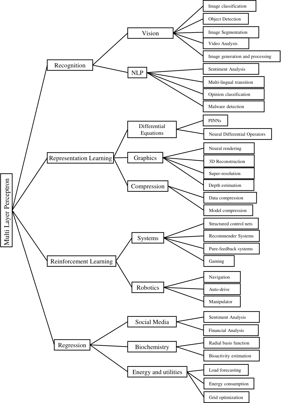
Fig. 1: Taxonomy categorizing various applications of MLP. Each category has multiple subcategories that illustrate the specific tasks and domains that MLP can address.

generated with our implementation for these applications are shown in Section IV.

Most MLP applications can be categorized into the following four categories:

• Recognition: using MLPs to identify objects, or patterns.

• Representation learning: aiming to extract meaningful patterns from raw data to create representations that are easier to understand and process by MLPs.

• Reinforcement learning: utilizing MLPs to learn from interactions with the environment to make better decisions.

• Regression: predicting values based on input data.

The taxonomy in Figure 1 categorizes contemporary MLP applications, which demonstrates the diversity and versatility of MLP in solving various real-world problems. We present these categories in the following sections in some detail.

A. Recognition

In vision, MLPs are applied to image classification [17]– [21], objects detection and semantic segmentation [22]– [26], video analysis [27]–[29], image processing and generation [30]–[33]. Other notable works in NLP include sentiment analysis and opinion classification [34]–[36], malware classification [37]–[39], adversarially robust [40] and multilingual transition [41] which leverages MLPs for language understanding and generation.

B. Representation Learning

MLPs may solve partial differential equations through Physics-Informed Neural Networks (PINNs) [4], [42]–[45] and neural differential operators [46]–[48], which approximate the solution to differential equations using neural networks.

In the field of neural graphics, MLPs have been developed and integrated into neural rendering [5], [49]–[53], 3D reconstruction [54]–[56], super-resolution [57] and depthestimation [58], [59]. In this work, we are interested in exploiting the potential of MLPs in the above three fields and will show their results in the Appendix A-C for details.

In the field of Compression, MLPs aim to reduce the size of data or models by removing redundant or irrelevant parameters and operations. MLPs are utilized to perform data compression by learning compact representations of data that can be reconstructed with minimal distortion [60], [61]. In addition, MLPs can be utilized for model compression by learning to approximate the function of large or complex models with smaller or simpler models [62], [63].

C. Reinforcement Learning

In the field of robotics, MLPs are integral for various tasks, including navigation [64]–[67], autonomous-driving [68], and manipulator [69]. In system research, MLPs have been employed for structured control nets [69], [70], recommender systems [71], [72], pure-feedback systems [73], [74] and Gaming [75], [76]. which utilize MLP-based deep learning techniques to discover system design and control.

D. Regression

Most existing works using MLPs on regression are in the fields of social media, biochemistry, and Energy.

In social media, MLPs play a pivotal role in sentiment analysis [77]–[80], financial analysis [81], [82] and fraud detection [83], [84], for analysis the social problems. Furthermore, in biochemistry research, MLPs are able to model complex biology and chemistry to explore the molecular basis of life in radial basis function [85] and bioactivity estimation [86]. In the field of energy and utilities, MLPs work well on load forecasting [87], energy consumption [88], and machine optimization [89] to deal with some biological issues and improve the effect of activities.

In the present section, we introduce our approach to the implementation of fully-fused MLPs on Intel GPUs. Section III-A we describe the inference and training algorithms. Section III-B then describes our SYCL joint matrix implementation for the Intel Data Center GPU Max 1550 in detail.

A. Inference and Training Operations

For the sake of conciseness and simplicity, we describe our implementation of fully-fused MLPs for the special case where the width of each layer, including input and output, is 64. Cases where the input and output size differs may be reduced to this special case by utilizing, e.g., encodings for the input data or appropriate padding of the data and the weights.

The matrix operations during training and inference are described in what follows. Let denote the batch size and let N = K = 64 denote the layer width. Let denote an activation function [90]. We use the notation , for a matrix A, to indicate the element-wise application of the activation function to the matrix A. Let denote the number of layers in the MLP, which includes the input and the output layer. I.e., it denotes the number of matrices as in Alg. 1. Further, let , , and denote matrices for each i = 1, . . . , nlayers. The transpose of any matrix A is given by . An element of a matrix A with the row coordinate r and the column coordinate c is given by . The matrices denote weights of each layer i,

1 ≤ i ≤ nlayers − 1.

A pseudo code of the inference is shown in Algorithm 1, which consists of repeated matrix multiplications and applications of the activation function .

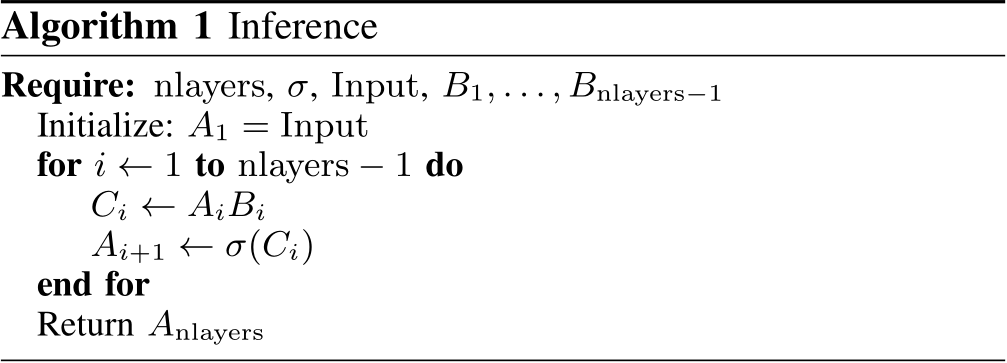
Our implementation of the inference step is based on several observations. First, each weight matrix fits in the shared local memory (SLM) [91] of the targeted Intel Data Center GPU Max 1550. The loads of the matrices from global memory, i.e., high bandwidth memory (HBM), can therefore be minimized by pre-fetching them one after the other into SLM. Secondly, up to eight rows of the matrices and (for a single i) fit into the general register file (GRF) for all network widths which are 64 or less. For network widths between 64 and 128, it still holds but requires large GRF mode [92]. This is relevant since the targeted XMX hardware may be applied to sub-matrices with up to eight rows. However, as analyzed in the following Sec. III-C, the highest arithmetic intensity is achieved when using sub-matrices consisting of exactly eight rows. Lastly, only and for a single i are required at the same time and only the last matrix is returned. The matrices associated with other layers are discarded during inference thus minimizing the amount of memory accesses required, consequently increasing the arithmetic intensity and performance.

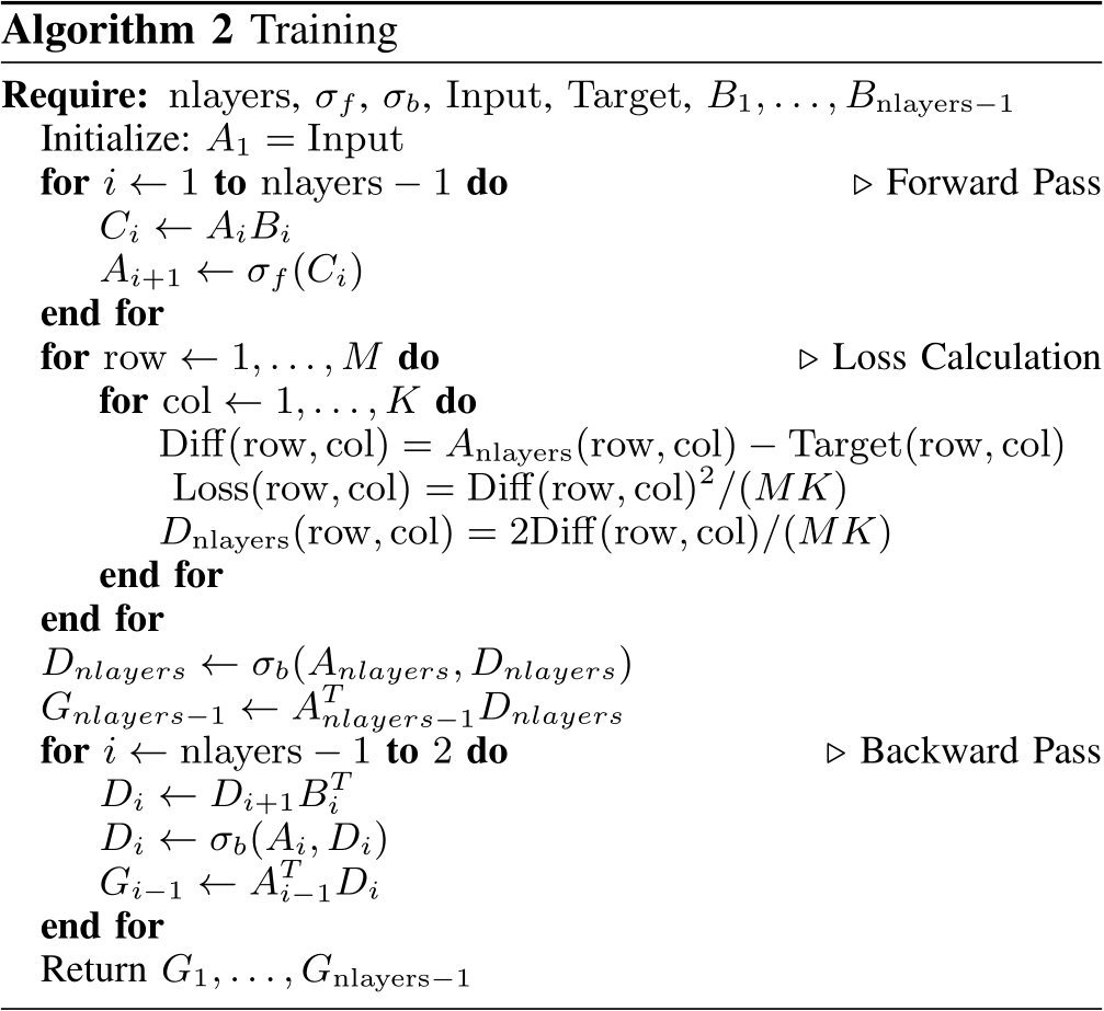
The pseudo code for the training of the network is shown in Algorithm 2. In particular, we focus on the forward pass and the subsequent backward pass after a loss is calculated. We do not consider the optimization step in this pseudo code. In contrast to the inference, the training takes as input two activation functions. One for the forward pass and one for the backward pass denoted by and , respectively. Note, that the activation function is the derivative of resulting from the chain rule during back-propagation [93]. In addition, the loss computation requires target values given as an array of real values, named Target. The outputs of the training algorithm are matrices . The matrices represent the gradients of the weight matrices . The gradients are required for the subsequent optimization step, which is typically some type of gradient descent algorithm and is a real square matrix of size (note that K = N as we have fixed layer widths of

2i, i = 4, ..., 7) .

The forward pass in Algorithm 2 is nearly identical to the inference. The only difference is that all matrices , i = 1, . . . , nlayers, have to be stored since they are required for the backward pass. The loss calculation in Algorithm 2 is an exemplary L2 loss. Note, that the loss calculation is explicitly mentioned as Loss(row, col) for illustration purposes but not stored as the derivative of the loss is used for the back-propagation step (see step i) in the following paragraph).

The backward pass consists of three steps: i) propagating the gradient backward to the next layer, ii) calculate the gradient of the loss with respect to the weighted inputs, and iii) calculate the gradient of the loss with respect to the weights. As follows from the chain rule for back-propagation, i) in each layer i the gradient propagation is realized as matrix multiplications between the matrix and the transpose of the weights matrix , ii) gradients with respect to weighted inputs are calculated as activation of the previous layer, and iii) gradients with respect to the weights are a matrix multiplication between the transpose of the forward outputs and the activated output of the backward pass. For a derivation of the backward pass, please refer to Chapter 6.5 in [93].

Our implementation of the training computes the forward pass, the loss and the backward pass within the same kernel to maximize the re-use of cached data and registers. Only the product is not part of our training kernel, although the time required for it is included in all of the performance data presented in the following Section IV. We found that it is in general preferable to launch a separate kernel for the products due to the differing dimensions of the matrix multiplications. In detail, a possible version which fuses the matrix multiplications into the training and which reuses the data already in the GRF would perform a block outer product of a block row in the matrix with a block row at the same position in the matrix to compute a partial sum of the whole output matrix. A subsequent reduction over all work-items would then be necessary for the final result. At the time of writing, we were not able to find an efficient implementation of the above approach or any other approach to the fusing of the product . We instead found that performing the operations with the highly optimized matrix-multiplication routines in Intel’s oneMKL, in a separate kernel after our training implementation finishes, delivers the best results.

B. SYCL joint matrix Implementation of MLPs

Our SYCL implementation is based on Intel’s joint matrix extension [9] to write code which can be executed on Intel’s XMX hardware [94] for the matrix multiplications. Efficient utilization of the XMX hardware is highly relevant since the theoretical multiply-add (MAD) peak performance of an Intel Data Center GPU Max 1550 on the targeted bfloat16 [95] (bf16) data type is approximately 838 tera floating point operations per second (Tflops/s), which is sixteen times the theoretical peak single-precision MAD throughput (Tflops/s) when utilizing the vector engines [94].

The Intel SYCL extension provides a joint matrix object, which represents a matrix of a small and fixed size distributed across a SYCL sub-group [9], and several related functions to facilitate computations with these joint matrix objects. In particular, we utilize the function joint matrix mad, which takes three joint matrices, say A, B, and C, and returns the joint matrix resulting from the operation AB + C, which is performed on the XMX hardware.

The joint matrix mad function is only available for specific matrix sizes. In detail, the matrix A has to be of size where can be chosen arbitrarily and TK depends on the device and the data type [96]. For the targeted bfloat16 data type, TK = 16 is required. The matrix B, in turn, has to be of size , where TN is device dependent. For the Intel Data Center GPU Max the value TN = 16 is required. The matrix C as well as the output matrix of the joint matrix mad function have to be of size . It is important to note that joint matrix mad performs the accumulation in single precision when utilizing bfloat16 for the inputs A and B. The matrix C and the output of the function are therefore of type float.

In the following detailed description, we focus on the inference (cf. Alg. 1) for the special case where K = N = 64. We launch the kernel with work-items, a sub-group size of 16 and a work-group size of 1024 work-items, i.e., the maximum possible work-group size to minimize the loads from HBM as discussed in the following Section III-C. Each sub-group with id sg id, sg id = 1, . . . , M/TM loads a unique block-row from the input into the register file starting at the row consisting of TM rows and K columns. Each sub-group stores this block-row as four joint matrix objects, each of size . In each layer i, each work-group (consisting of 64 sub-groups) loads the weight matrix jointly from HBM into SLM. At the end of the algorithm, each sub-group stores its TM rows of the matrix to HBM.

Figure 2 illustrates the loads to the register file (green) per sub-group and the joint load to SLM (blue) per work-group for a single layer i. Each sub-group then computes the product of its block-row with the weights matrix and keeps the resulting four joint matrix objects (K = 64, TK = 16) in the registers. The weight sub-matrices sized , which are required to facilitate the joint matrix mad function, are loaded on-the-fly from SLM as needed using the joint matrix load [97] function. The weights are stored in a packed format [98] to increase the performance of the load.

After the matrix-matrix product, each sub-group applies the activation function to its resulting block-row and utilizes the output of the activation function in the next iteration as input to the subsequent matrix-matrix product. Thus, it keeps the data in the register file and avoids accesses to HBM or caches. This idea is similar to [6]. However, our approach keeps the weights matrix in SLM and the input and output in the registers. Our algorithm requires two local synchronizations per layer due to the utilization of the SLM for the weights. The first synchronization ensures that the copy of the weight matrix into SLM is finished before accessing it. The second synchronization is to ensure that every work-item in the work-group finished accessing the weight matrix in SLM before starting the copy the weight matrix for the next layer.

The training algorithm 2 is similar to the inference described above and follows the same structure. Although, in contrast to the inference, each layer i in the training has to store the matrices and , which may impact the performance. As indicated above, the final matrix-matrix multiplications, , are performed by oneMKL outside of our training kernel since no fusing is possible for these operations.

To conclude this section, we discuss the limitations of our approach and propose mitigation strategies.

First, to achieve an occupancy of 100% on the Intel Data Center GPU Max 1550, 8192 sub-groups have to be launched. Thus, problems with a batch size of less than (TM = 8) do not fully occupy the device with our strategy and show reduced performance. This restriction is alleviated by choosing a smaller value for TM, which

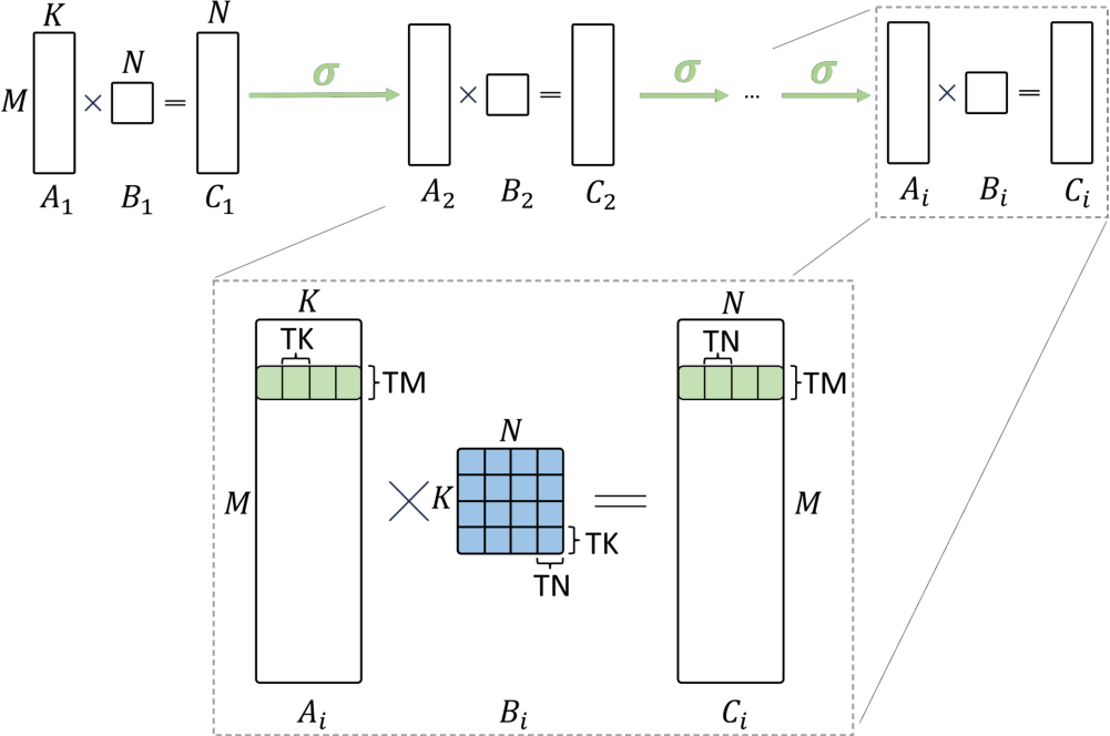
Fig. 2: Illustration of our implementation. On the left handside, all multiple layers are sketched. Each layer is parallelized along the batch size (i.e., the M dimension). The right handside sketches a single layer. The data of a single sub-group is colored. Green indicates data in the register file. Blue indicates data in the SLM. Each sub-group performs a matrix-matrix multiplication of size utilizing joint matrix objects of size , and .

increases the number of launched sub-groups. As discussed in Section III-C this reduces the arithmetic intensity and may lead to a higher occupancy at the cost of a lower arithmetic intensity.

Secondly, due to the fixed dimensions of the inputs to the joint matrix mad functions, the batch size M has to be a multiple of TM and the network width N = K has to be a multiple of TN and TK. This limits the possible width of the network to multiples of 16 on the Intel Data Center GPU Max 1550. These limitations can be removed by simply padding the batch size to the next multiple of TM and the network width to the next multiple of 16. Another alternative would be to use two-dimensional load functions and hardware-supported zero-padding of out-of-bounds accesses for these two-dimensional loads. Although, at the time of writing, support of two-dimensional loads is currently lacking in Intel’s SYCL implementation and may required to use intrinsics and built-in functionalities.

Finally, our algorithm is based on storing whole blockrows in the register file. The maximum possible width of the network is therefore determined by the size of the register file and given as 128 elements when utilizing the large register mode [92]. In fact, assuming that the sizes of the data types of the inputs, the weights, and the output of each layer are given as, say, , and bytes, respectively, we allocate bytes per sub-group in the register file at the same time to facilitate the joint matrix multiplications (3584 bytes for N = K = 64, , and .) While the default size of the register file of the Intel Data Center GPU Max 1550 is 8192 bytes per sub-group, i.e., more than twice the size required for the joint matrix multiplications, we empirically found that a width larger than 64 elements does not fit in the GRF and thus results in register spills. Although, the register allocation depends on the driver version and may change in the future. Since the large register mode doubles the GRF size, MLPs with a width of 128 elements fit. The register pressure may be reduced by choosing a smaller value for TM at the cost of performance (see following Section III-C for the relation between TM and the arithmetic intensity).

C. Roofline Analysis

Similar to [6], our goal is to minimize the accesses to the relatively slow HBM. To analyze how well our implementation achieves this goal, we compare our implementation to the CUDA implementation in [6] utilizing a roofline model [99] with bandwidth limits. We compute and compare the arithmetic intensities of the algorithms for TM = 8, K = N = 64 and the bfloat16 data type (i.e., 2 byte per value in memory). A higher arithmetic intensity indicates that more floating point operations per byte can be performed and thus shows that the performance is less limited by the memory bandwidth. Note, that a higher arithmetic intensity does not necessarily translate to a higher throughput since other factors (e.g. latency, frequency throttling, etc.) may be limiting the performance. Further note, that we are not considering the floating point operations performed by the activation function in the following analysis.

We use 1024 work-items per work-group and a sub-group size of 16 work-items. Thus 64 sub-groups (1024/16) constitute one work-group. The number of loads of the weights matrix from HBM is inversely proportional to the number of sub-groups in a work-group (see Section III-B). As each sub-group computes TM rows of the M rows of the input, we launch M/TM sub-groups or workgroups. Each work-group has its own SLM and thus each work-group needs to load the weights matrix from HBM into its SLM. Note, that in our particular case the weights matrix may be cached in L2. We neglect the effects of the L2 cache in our roofline analysis, as it would depend on too many parameters, including N, K, M, TM, nlayers, and datatypes.

As a consequence, for a single layer 1, under the above mentioned assumption that none of the data is cached in the L2 cache, our algorithm loads bytes from HBM to facilitate a matrix-matrix product of flops for an arithmetic intensity of flops per byte loaded from HBM. For our choice of TM = 8 our algorithm thus achieves an arithmetic intensity of 512 flops per byte loaded from HBM for the matrix-matrix product in every hidden layer, i.e., all layers except the input and output layers (where additional loads of the input from HBM or stores of the output to HBM are required). Together with a HBM bandwidth of approximately 2 TB/s (theoretical peak is TB/s, 2 TB/s is a realistic bandwidth for complex workloads), this shows that the arithmetic intensity is high enough such that the available HBM bandwidth is not a limiting factor and that each layer is compute bound.

Analogously, the tiny-cuda-nn implementation presented in [6] loads the weight matrix for each layer i, i = times from HBM (again discarding that the values may be cached in the L2 cache). This results in an arithmetic intensity of 128 flops per byte loaded from HBM. The Nvidia H100 PCIe GPU delivers a theoretical peak HBM bandwidth of approximately 2 TB/s [13]. The theoretical peak throughput of the tiny-cuda-nn inference algorithm is thus reduced to 256 Tflops/s. Each layer in the CUDA implementation is therefore bound by the HBM bandwidth.

Extending the above model to consider the whole inference algorithm, including the loads of the input data and stores of the output, we get the following arithmetic intensities (also known as operational intensities; abbreviated as OI to prevent confusion with AI – Artificial Intelligence) in dependence of the number of layers:

For example, for a number of nlayers = 6, the arithmetic intensity of the SYCL implementation is 121.9 flops per byte, limiting the theoretical peak performance to approximately 243.8 Tflops/s. The arithmetic intensity for the CUDA implementation is 71.1 flops per byte, resulting in a theoretical peak performance of approximately 142.2 Tflops/s.

Further extending the above model to the forward pass in the training step, where each is additionally stored in HBM, we get an arithmetic intensity of flops per byte for the SYCL implementation (flops per byte for Tflops/s) and 1)/(3nlayers + 1) for the CUDA implementation (flops per byte for Tflops/s) thus further reducing the theoretical peak performance for both codes.

Finally, considering the forward pass and the backward pass (loading the input, storing each and once, loading and according to the work-group size and the batch size, loading and once for the final calculation of the ) results in theoretical peak performance as displayed in Fig. 3.

Similar considerations as above for the accesses to SLM lead to an arithmetic intensity of 7.877 flops per byte accessed in SLM for the SYCL implementation and 25.6 flops per byte for the CUDA code. Thus, based on the theoretical peak SLM bandwidth of the targeted device, the SLM accesses limit the performance of our SYCL code to 393 Tflops/s (instead of 838 Tflops/s). This is never an issue for the training since the HBM bandwidth imposes a lower limit on the performance than the SLM bandwidth. Although, the SLM bandwidth limits the performance for the inference to at most to 393 Tflops/s when .

To emphasize the advantages of fused MLPs compared to non-fused MLPs, we compare the above arithmetic intensities to the arithmetic intensities of non-fused implementations in what follows. A non-fused implementation of the inference algorithm 1 would require for each layer a load of the matrices

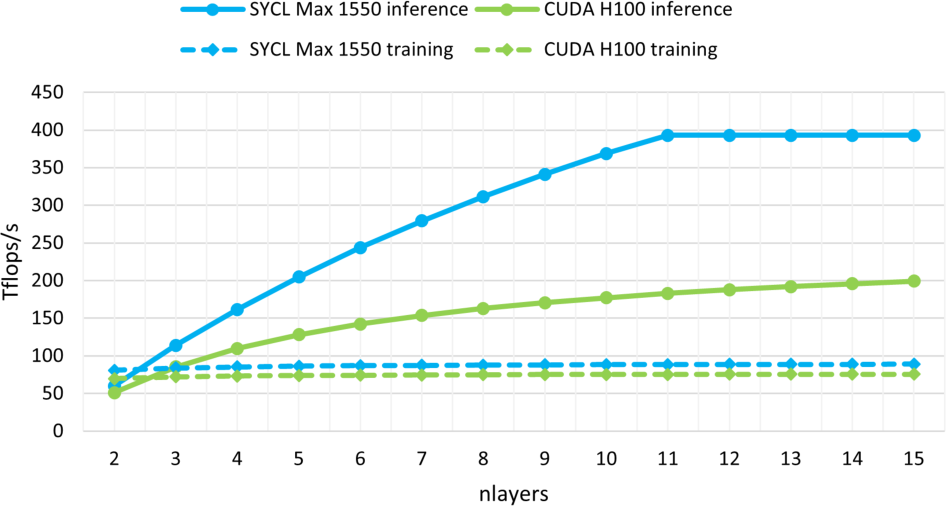
Fig. 3: Comparison of the theoretical peak performance based on the the roofline analysis in Section III-C.

and with a subsequent store of to facilitate a single matrix-matrix product. Thus, the arithmetic intensity is bounded by 32 flops per byte loaded (independent of the number of layers) for the inference, which is up to 1/16-th of the arithmetic intensity of a fused implementation. Similar considerations for the training show that the fused training only increases the arithmetic intensity by up to a factor 2 at most (in the limit ).

To summarize, Figure 3 shows the theoretical peak performance based on the above roofline analysis for the CUDA implementation on Nvidia’s H100 GPU and the SYCL implementation on Intel’s Data Center GPU Max 1550. It shows that our algorithm improves the theoretical peak performance of the CUDA implementation [6] by increasing the arithmetic intensity for the HBM accesses and that decreasing the arithmetic intensity for SLM accesses does not have a negative impact. The performance which may be achieved in practice is discussed in the following Sec. IV.

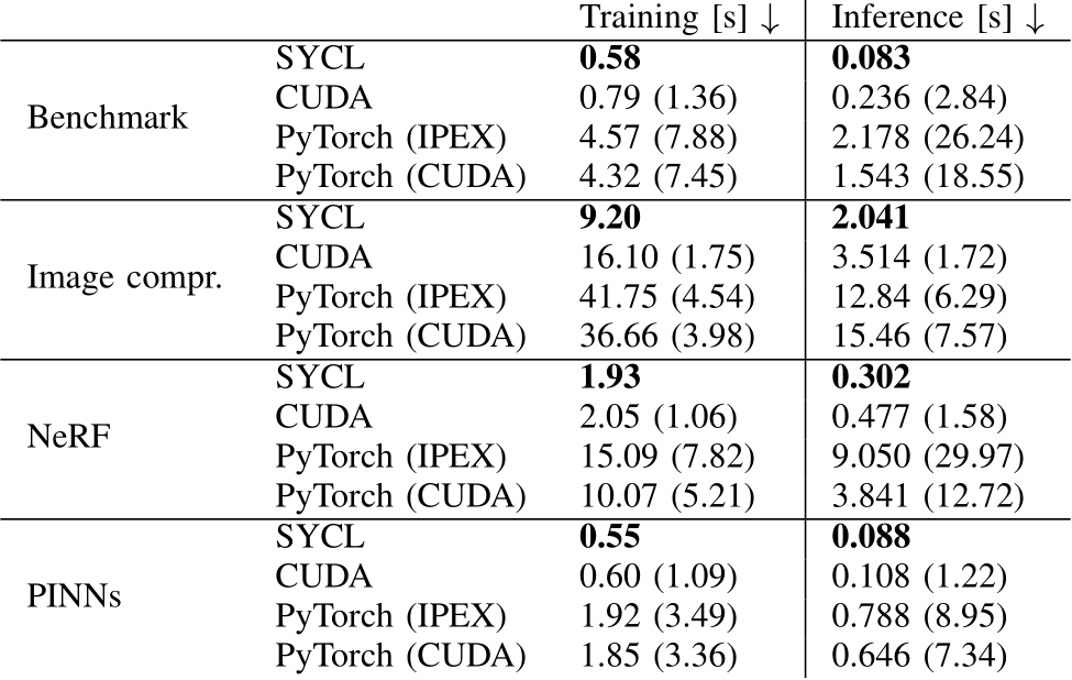
In this section, we demonstrate how our fully-fused MLP implementation increases the performance of four commonly used AI tasks: non-linear function approximation, image compression, Neural Radiance Fields (NeRFs), and solving differential equations with PINNs (see Section II). For every comparison, we compare our SYCL implementation on an Intel Data Center GPU Max 1550 with the CUDA implementation [8] on a Nvidia H100 GPU and PyTorch using both Intel Extension for PyTorch (IPEX) [12] and CUDA backend. The results of the comparison can be seen in Table I.

To ensure a fair comparison of the forward and backward performances and to disregard differences in the implementation of the loss functions and optimiser, we only measure the time of the code where the fusion of the operators is relevant for, i.e., forward and backward calculation (cf. Algs. 1, 2). The benchmark protocol is identical for both implementations: every forward and backward pass is called for the same amount of episodes, the same batch sizes, MLP architecture, and ReLU activation functions and a linear output activation function.

TABLE I: Training and Inference times for our implementation (SYCL), the fully-fused implementation from [6] (CUDA) and PyTorch using both IPEX and CUDA. The numbers in the brackets indicate the time relative to our implementation.

The CUDA implementation [8] is tested on a dual-socket system with two Intel Xeon Platinum 8480+ CPUs, 512GB DRAM and Nvidia H100 GPUs with Ubuntu 22.04 LTS as operating system. The code was compiled with CUDA version 12.3.52 (nvcc version built on Sept. 8 19:17:24PDT 2023). The driver version is 535.129.03.

The SYCL code, on the other hand, is tested on a dual-socket system with two Intel Xeon Platinum 8480+ CPUs, 512GB DRAM and Intel Data Center GPU Max 1550 GPUs with Ubuntu 22.04.3 LTS as operating system. We utilized the mpiicpx compiler (Intel oneAPI DPC++/C++ Compiler 2023.2.0 (2023.2.0.20230721)) included in the oneAPI 2023.2 toolkit and an unreleased engineering driver*. To scale our implementation to both Xe Stacks [94] in an Intel GPU, we use Intel MPI version 2021.10.0.

A. Non-linear Function Approximation

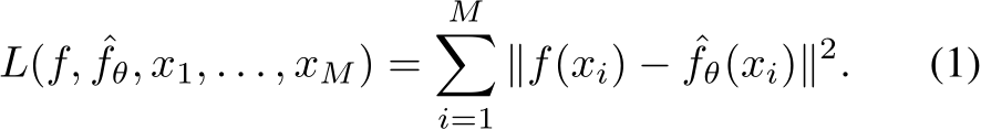
The goal of non-linear function approximation is to train a Neural Network to approximate a given non-linear function . During the training the residual loss between target function f and approximation is typically chosen as the mean square error, which is depicted in what follows for a batch size M:

In this section, the performance of our SYCL implementation is compared to the CUDA implementation [8] for various batch sizes M. To determine relevant batch sizes, we investigated the distribution of batch sizes used in MLP-based methods [4], [42], [43], [45]–[47], [49]–[53], [58], [100]– [104], [104]–[119], [119]–[127] in the fields of NeRFs, Neural Compression, and PINNs mentioned in Appendix A- C. The results of this investigation are summarized in Table II. The distribution appears to be approximately normal, with the majority of batch sizes falling between and suggesting that many MLP-based methods in these fields use large batch sizes, where our fully-fused implementation reaches maximal occupancy and performance (see Fig. 4).

TABLE II: Batch Sizes of commonly used MLP applications

For NeRFs, the batch size is the number of rays per batch and corresponding samples per ray during ray tracing. We the formula in [128] to calculate the batch size: number of rays per batch number of samples per ray for the full method. For Neural Compression, and Partial Differential Equations (PDEs), since many methods in these representation learning use full-batch gradient descent as the training strategy, we adopt the dataset size as the full batch size for both the training and inference steps.

Based on this data, batch sizes larger than elements are not commonly used and thus not considered in this test. Small batch sizes, in turn, are also removed from the test since the occupancy decreases proportional to the batch size for batch sizes smaller than (cf. Sec. III-B). The performance is thus limited by the occupancy and fusing the operations does not provide any benefit.

In our test we learn an MLP that approximates a non-linear function . We measure the throughput for our SYCL implementation on a single Xe Stack and both Xe Stacks of an Intel Data Center GPU Max 1550 and compare the results to the throughput measured with the CUDA implementation [8] on a Nvidia H100 GPU. For both implementations, we use a network width of 64 with input and output width of 64 elements. As indicated above, the batch size M varies from to , and we run the benchmark for niter iterations calculated as niter = max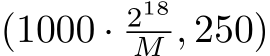. Further, we choose four hidden layers, i.e., nlayers = 6.

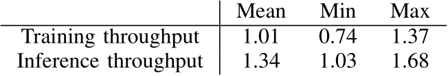
The resulting performance graphs for training and inference can be seen in Figure 4 and the relative performance gain of our method compared to CUDA can be seen in Table III. The figure shows that the performance in the training case (bottom graph of Fig. 4) is similar for both implementations. This coincides well with the roofline predictions from Section III-C. It is also interesting to note that the peak performance of approximately 70 Tflops/s is close to the roofline prediction of Tflops/s thus indicating that the problem is indeed bound by the HBM bandwidth.

TABLE III: Relative Performance Gain of SYCL compared to CUDA for Function Approximation

The inference results (top graph of Fig. 4), in contrast, show that the SYCL implementation outperforms the CUDA implementation. For the smaller batch sizes even when utilizing only half of the Intel device. This coincides again well with the

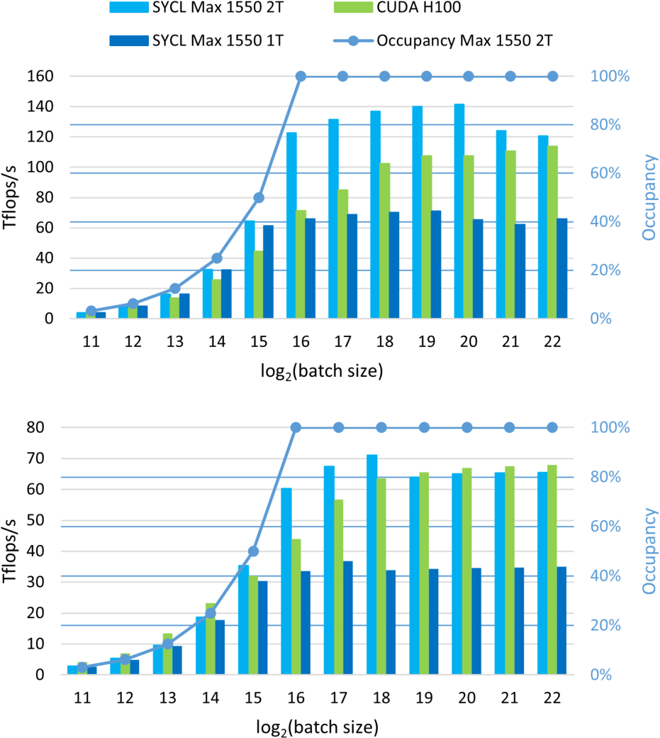
Fig. 4: Performance of the inference (top) and training (bottom) of our SYCL implementation on a single tile of the Intel Data Center GPU Max 1550 (dark blue) and two tiles of the same Intel GPU (light blue) compared to the CUDA code on a Nvidia H100 GPU (green) for nlayers = 6. The occupancy of the SYCL code on the two tiles of the Intel Data Center GPU is given as the blue line. The x-axis denotes the batch size (i.e., M) from inputs to .

roofline analysis in Section III-C. Although, the measured peak performance of approximately 140 Tflop/s falls short of the predicted Tflops/s. Our performance investigations have shown that this is due to scoreboard ID stalls occurring when loading the weights matrices from SLM thus indicating that the performance of our problem is not bound by the memory bandwidth but by the SLM memory latency. Investigation how to eliminate this latency are ongoing.

To fully show demonstrate the performance of our approach, we measure the time required to calculate 1000 iterations for non-linear function approximation using an MLP of 11 hidden layers and network width of 64. The batch size is chosen as . The results can be seen in the Benchmark row of Table I. Our SYCL implementation reaches performance gains of up to 7.88 times faster, and up to 26.24 times faster for training and inference respectively.

As mentioned in Section III-B, the Intel GPU is not fully occupied for batch sizes smaller than resulting in reduced performance. Note that maximum performances for the SYCL implementation are not achieved for the largest batch sizes, but for those batch sizes where the occupancy is maximal while the problem is sufficiently small to fit in the L2 cache.

B. Image Compression

For Image Compression, the MLP learns the color distribution of an image represented as function that maps from 2-D coordinates (pixels) to corresponding color. We use a network width of 64. As NNs poorly learn high-frequent details of the target function f, encodings are typically used to mitigate this issue. Encodings pre-process the 2D pixel input by directly mapping them into a spectrum of high-frequent signals, which are then fed into the MLP. The Multiresolution hash encoding [128] is used, which can be seen as the input to the MLP. The final function approximator is thus , with Multiresolution Hash Encoding g and MLP .

The learning progress can be seen in Figure 5. We used a network width of 64 with input 32, output width 1, and batch size for 1000 iterations. After 10 steps the colors are not entirely correct, but the silhouette is recognisable. Then, over the next 900 steps, the colors and finer details are becoming gradually clearer until the training progress converges after 1000 steps. The whole training takes 9.2s for the SYCL implementation and is 1.75 faster than the CUDA implementation and 4 times faster than PyTorch. The image can be reconstructed (inference) within 2.41s for SYCL (see row Image compr. in Table I).

For comparison, storing the image at a resolution of 3072 with greyscale values costs 2.3MB for a JPEG image, while storing 12288 half precision weights costs 25 kb.

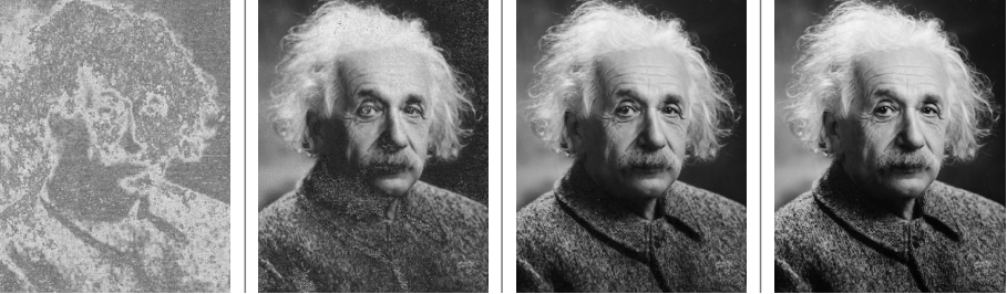
Fig. 5: Training progress of Image Compression. The training converges after 1000 steps. The training and inference process is performed for both the SYCL and CUDA implementation and the visualised progress if implemented as per [8].

C. Neural Radiance Fields (NeRF)

For NeRFs, the goal is to learn a Radiance Field (see Appendix A) . Similar to Image Compression, NeRFs require an encoding as input to the MLP for better representations of the high-frequent details of the object. Multiresolution hash encoding is used for this task resulting in a 32-dimensional feature vector as input to the MLP. A network width of 64 is chosen with input width 32, output width 4, and a batch size K = 1048576. For details about the implementation of the NeRF algorithm, please see [129].

The training of the MLP without encoding and volume rendering is conducted within 1.93s for training and 0.302s inference in our SYCL implementation. Compared to the CUDA implementation, this is 1.06 and 1.58 times faster for training and inference respectively. The generated images can be seen in Figure 6.

D. Physics-Informed Neural Networks (PINN)

To demonstrate how our method can be applied to solve Partial Differential Equations (PDE), we leverage the PINNs framework [123] to train an MLP that represents the solution of the following two-dimensional Navier-Stokes Equation:

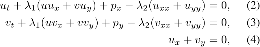
with velocity fields u(t, x, y) and v(t, x, y) for the x and y components respectively, pressure p(t, x, y), and unknown parameters . For more details of the problem, please refer to Section 4.1.1 in [123].

We used DeepXDE [130] to find the PINNs f(t, x, y), g(t, x, y) that represent the solution of the Navier stokes equations (2). For details, see Appendix C.

The dataset and thus batch size consists of data points. For 1000 iterations, the training time takes 0.55s for SYCL, 0.60s for CUDA yielding a performance gain of up to 3.49 compared to PyTorch. The evaluation of the PDE solution on collocation points requires 0.088, which results in an improvement of up to 8.95x.

In this paper, we presented a SYCL implementation of fully-fused Multi-Layer Perceptrons (MLPs) on Intel Data Center GPU Max. Our approach focuses on maximizing data reuse within the general register file and the shared local memory, minimizing the need for slower global memory accesses. This results in a significant increase in the arithmetic intensity, which leads to improved performance, especially for inference.

Our implementation outperforms an equivalent CUDA implementation for MLPs with width 64 by a factor of up to 2.84 in inference and 1.75 in training in our tests, demonstrating the effectiveness of our approach, and outperforms the PyTorch implementation by up to a factor of 30. We further showcased the efficiency of our implementation in three significant areas: Image Compression, Neural Radiance Fields (NeRF), and Physics-Informed Machine Learning. Across all these domains, our approach demonstrated substantial improvements, achieving factors up to 30 times when compared to conventional PyTorch implementations and up to 2.84 times over highly optimized CUDA implementations.

In the future, we aim to further optimize our implementation. A strong focus will be a more efficient usage of registers which may enable further prefetching of the weights matrices, thus reducing the stalls. In addition, we may be able to reduce the utilization of SLM and enable the loads of multiple weights matrices in the SLM, which would reduce the number of necessary barriers. Another important aspect will be to increase the occupancy for small batch sizes by either increasing the arithmetic intensity for smaller values of TM or by partitioning the work along the K dimension, which requires the usage of atomic operations. Lastly, an important optimization would be the fusion of the final matrix products

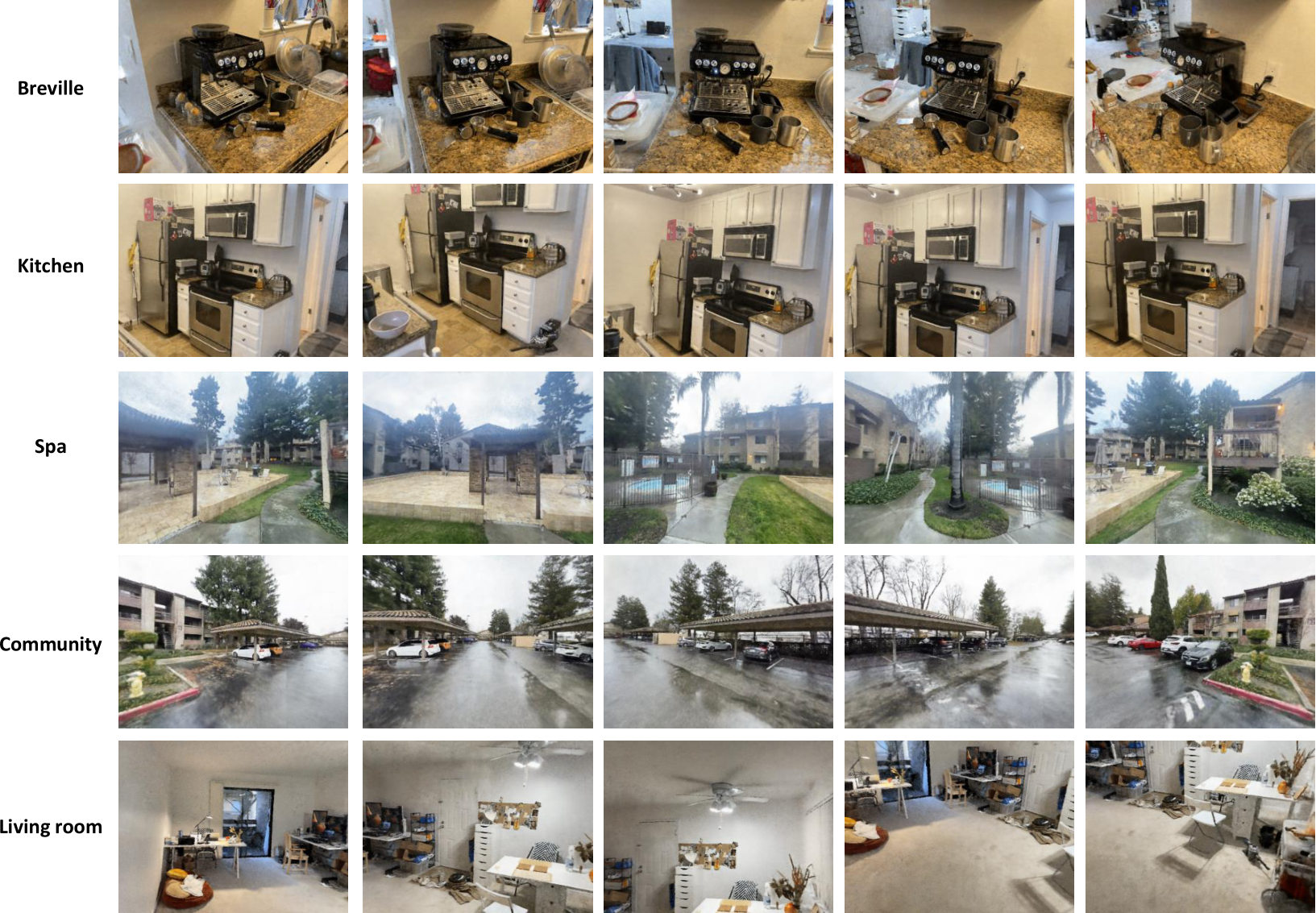
Fig. 6: CLNeRF results on 5 scenes for breville, kitchen, spa, community, and living room. Each row represents a different scene and each column shows the scene rendering results from different views using the MLP as NeRF.

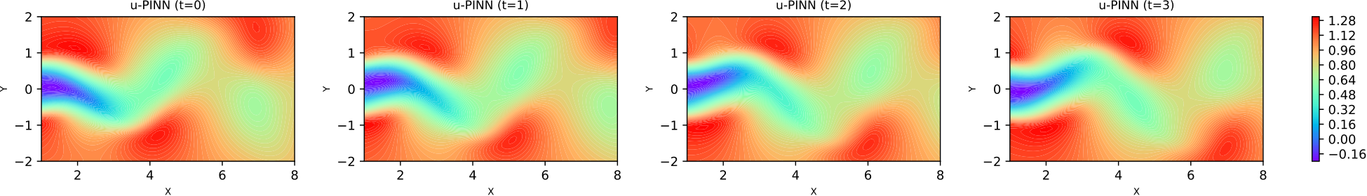
Fig. 7: Visualisation of learned solution to Navier Stokes Equation. Mean Absolute Percentage Error: 0.1%. Results generated using DeepXDE [130].

(cf. Alg. 2) into the backward pass. It could potentially increase the performance of the training by up to a factor 2, based on the roofline model.

Our implementation is open-sourced to allow for wider usage and contributions from the community. The code can be found at https://github.com/intel/tiny-dpcpp-nn.

In addition to further performance optimization, we also plan to explore the use of Intel’s ESIMD SYCL extension for our implementation and compare it to our existing SYCL implementation. Our past experience with ESIMD showed that it enables a better control over the register usage and exposes cache controls for load and store operations.

In future work, we aim to generalize our library to various data types and larger network widths. In addition, we plan to

implement an optimized version for Intel’s Arc GPUs.

ACKNOWLEDGMENT We’d like to thank Jia Xu and Jing Xu for their help and advise during the development of tiny-dpcpp-nn.

DISCLAIMERS Performance varies by use, configuration and other factors. Learn more on the Performance Index site. Performance results are based on testing as of dates shown and may not reflect all publicly available updates. No product or component can be absolutely secure. Your costs and results may vary. Intel technologies may require enabled hardware, software or service activation.

©Intel Corporation. Intel, the Intel logo, and other Intel marks are trademarks of Intel Corporation or its subsidiaries. Other names and brands may be claimed as the property of others.

[1] B. Yegnanarayana, Artificial neural networks. PHI Learning Pvt. Ltd., 2009.

[2] A. Vaswani, N. Shazeer, N. Parmar, J. Uszkoreit, L. Jones, A. N. Gomez, Ł. Kaiser, and I. Polosukhin, “Attention is all you need,” Advances in neural information processing systems, vol. 30, 2017.

[3] Z. Li, F. Liu, W. Yang, S. Peng, and J. Zhou, “A survey of convo- lutional neural networks: analysis, applications, and prospects,” IEEE transactions on neural networks and learning systems, 2021.

[4] S. Cuomo, V. S. Di Cola, F. Giampaolo, G. Rozza, M. Raissi, and F. Piccialli, “Scientific machine learning through physics-informed neural networks: Where we are and what’s next,” Journal of Scientific Computing, vol. 92, no. 88, pp. 1–35, 2022.

[5] B. Mildenhall, P. P. Srinivasan, M. Tancik, J. T. Barron, R. Ramamoor- thi, and R. Ng, “Nerf: Representing scenes as neural radiance fields for view synthesis,” Communications of the ACM, vol. 65, no. 1, pp. 99–106, 2021.

[6] T. M¨uller, F. Rousselle, J. Nov´ak, and A. Keller, “Real-time neural radiance caching for path tracing,” arXiv preprint arXiv:2106.12372, 2021.

[7] S. Park, C. Yun, J. Lee, and J. Shin, “Minimum width for universal approximation,” arXiv preprint arXiv:2006.08859, 2020.

[8] T. M¨uller, “tiny-cuda-nn,” 4 2021. [Online]. Available: https: //github.com/NVlabs/tiny-cuda-nn

[9] Intel Corporation. (2023) Programming Intel® XMX using SYCL: Joint Matrix Multiplication. Intel oneAPI Optimization Guide for GPU. [Online]. Available: https://www.intel.com/ content/www/us/en/docs/oneapi/optimization-guide-gpu/2024-0/ programming-intel-xmx-using-sycl-joint-matrix.html

[10] J. Peddie, “The sixth era gpus: Ray tracing and mesh shaders,” in The History of the GPU-New Developments. Springer, 2023, pp. 323–360.

[11] H. Jiang, “Intel’s ponte vecchio gpu: Architecture, systems & software,” in 2022 IEEE Hot Chips 34 Symposium (HCS). IEEE Computer Society, 2022, pp. 1–29.

[12] Intel Corporation, “Intel extension for pytorch,” https://github.com/ intel/intel-extension-for-pytorch, 2023, gitHub repository.

[13] Nvidia Corporation. (2023) H100 Tensor Core GPU. [Online]. Available: https://www.nvidia.com/en-us/data-center/h100/

[14] R. Liu, Y. Li, L. Tao, D. Liang, and H.-T. Zheng, “Are we ready for a new paradigm shift? a survey on visual deep mlp,” Patterns, vol. 3, no. 7, 2022.

[15] W. H. Delashmit, M. T. Manry et al., “Recent developments in multilayer perceptron neural networks,” in Proceedings of the seventh annual memphis area engineering and science conference, MAESC, 2005, pp. 1–15.

[16] M.-H. Guo, Z.-N. Liu, T.-J. Mu, D. Liang, R. R. Martin, and S.-M. Hu, “Can attention enable mlps to catch up with cnns?” Computational Visual Media, vol. 7, pp. 283–288, 2021.

[17] Q. Hou, Z. Jiang, L. Yuan, M.-M. Cheng, S. Yan, and J. Feng, “Vision permutator: A permutable mlp-like architecture for visual recognition,” IEEE Transactions on Pattern Analysis and Machine Intelligence, vol. 45, no. 1, pp. 1328–1334, 2021.

[18] X. Ding, C. Xia, X. Zhang, X. Chu, J. Han, and G. Ding, “Repmlp: Re-parameterizing convolutions into fully-connected layers for image recognition,” in Proceedings of the IEEE/CVF Conference on Computer Vision and Pattern Recognition, 2022.

[19] Y. Rao, W. Zhao, Z. Zhu, J. Lu, and J. Zhou, “Global filter networks for image classification,” in Advances in Neural Information Processing Systems, vol. 34, 2021.

[20] H. Touvron, P. Bojanowski, M. Caron, M. Cord, A. El-Nouby, E. Grave, G. Izacard, A. Joulin, G. Synnaeve, J. Verbeek et al., “Resmlp: Feedforward networks for image classification with data-efficient training,” arXiv preprint arXiv:2105.03404, 2021.

[21] H. Liu, Z. Dai, D. R. So, and Q. V. Le, “Pay attention to mlps,” arXiv preprint arXiv:2105.08050, 2021.

[22] S. Chen, E. Xie, C. Ge, R. Chen, D. Liang, and P. Luo, “Cyclemlp: A mlp-like architecture for dense prediction,” in Proceedings of the International Conference on Learning Representations, 2022.

[23] J. Lahoud and B. Ghanem, “2d-driven 3d object detection in rgbd images,” in Proceedings of the IEEE International Conference on Computer Vision, 2017, pp. 4622–4630.

[24] S. Pan, C.-W. Chang, T. Wang, J. Wynne, M. Hu, Y. Lei, T. Liu, P. Patel, J. Roper, and X. Yang, “Unext: Mlp-based rapid medical image segmentation network,” in Medical Image Computing and Computer Assisted Intervention – MICCAI 2022. Springer, 2022, pp. 23–33.

[25] L. An, L. Wang, and Y. Li, “Abdomen ct multi-organ segmentation using token-based mlp-mixer,” Medical Physics, 2021.

[26] H.-P. Lai, T.-T. Tran, and V.-T. Pham, “Axial attention mlp-mixer: A new architecture for image segmentation,” in 2022 IEEE Ninth International Conference on Communications and Electronics (ICCE). IEEE, 2022, pp. 381–386.

[27] Z. Qiu, T. Yao, C.-W. Ngo, and T. Mei, “Mlp-3d: A mlp-like 3d archi- tecture with grouped time mixing,” in Proceedings of the IEEE/CVF Conference on Computer Vision and Pattern Recognition, 2022, pp. 3062–3072.

[28] L. An, L. Wang, and Y. Li, “Morphmlp: An efficient mlp-like backbone for spatial-temporal representation learning,” Sensors, vol. 22, no. 18, p. 7024, 2021.

[29] J. Xia, M. Zhuge, T. Geng, S. Fan, Y. Wei, Z. He, and F. Zheng, “Skating-mixer: Long-term sport audio-visual modeling with mlps,” arXiv preprint arXiv:2203.03990, 2022.

[30] Z. Tu, H. Talebi, H. Zhang, F. Yang, P. Milanfar, A. Bovik, and Y. Li, “Maxim: Multi-axis mlp for image processing,” in Proceedings of the IEEE/CVF Conference on Computer Vision and Pattern Recognition, 2022, pp. 5769–5780.

[31] N. Sharma, R. Sharma, and N. Jindal, “New approaches to determine age and gender in image processing techniques using multilayer perceptron neural network,” International Journal of Computer Applications, vol. 164, no. 1, pp. 1–5, 2017.

[32] G. Cazenavette and M. Ladron De Guevara, “Mixergan: An mlp-based architecture for unpaired image-to-image translation,” arXiv preprint arXiv:2105.14110, 2021.

[33] Y. Mansour, K. Lin, and R. Heckel, “Image-to-image mlp-mixer for image reconstruction,” arXiv preprint arXiv:2202.02018, 2022.

[34] Z. Al-Makhadmeh and A. Tolba, “Improving sentiment analysis in arabic and english languages by using multi-layer perceptron model (mlp),” in 2020 IEEE 7th International Conference on Data Science and Advanced Analytics (DSAA). IEEE, 2020, pp. 1328–1334.

[35] J. Sultana, N. Sultana, K. Yadav, and F. AlFayez, “Prediction of sentiment analysis on educational data based on deep learning approach,” in 2018 21st Saudi Computer Society National Computer Conference (NCC). IEEE, 2018, pp. 1–6.

[36] Z. Al-Makhadmeh and A. Tolba, “Automatic hate speech detection using killer natural language processing optimizing ensemble deep learning approach,” Computing, vol. 102, pp. 501–522, 2019.

[37] T. K. Tran and H. Sato, “Nlp-based approaches for malware classifi- cation from api sequences,” in 2017 21st Asia Pacific Symposium on Intelligent and Evolutionary Systems (IES). IEEE, 2017, pp. 101–105.

[38] D. Dang, F. Di Troia, and M. Stamp, “Malware classification using long short-term memory models,” arXiv preprint arXiv:2103.02746, 2021.

[39] Y. Qiao, W. Zhang, X. Du, and M. Guizani, “Malware classification based on multilayer perception and word2vec for iot security,” ACM Transactions on Internet Technology (TOIT), vol. 22, no. 1, pp. 1–22, 2021.

[40] M. Raman, P. Maini, J. Z. Kolter, Z. C. Lipton, and D. Pruthi, “Model- tuning via prompts makes nlp models adversarially robust,” arXiv preprint arXiv:2303.07320, 2023.

[41] F. Fusco, D. Pascual, and P. Staar, “pnlp-mixer: an efficient all-mlp architecture for language,” arXiv preprint arXiv:2202.04350, 2022.

[42] T. Alkhalifah and X. Huang, “Physics informed neural learning of wavefields using gabor basis functions.”

[43] M. Takamoto, F. Alesiani, and M. Niepert, “Learning neural pde solvers with parameter-guided channel attention,” in Proceedings of the 38th International Conference on Machine Learning, 2023, pp. 9801–9811.

[44] H. Eivazi, M. Tahani, P. Schlatter, and R. Vinuesa, “Physics-informed neural networks for solving reynolds-averaged navier–stokes equations,” Physics of Fluids, vol. 34, no. 7, p. 075117, 2022.

[45] S. Wang, S. Sankaran, and P. Perdikaris, “Respecting causality is all you need for training physics-informed neural networks,” Journal of Scientific Computing, vol. 92, no. 88, pp. 1–35, 2022.

[46] L. Lu, P. Jin, and G. E. Karniadakis, “Deeponet: Learning nonlinear operators for identifying differential equations based on the univer-

sal approximation theorem of operators,” Journal of Computational Physics, vol. 404, p. 109108, 2020.

[47] L. He, Y. Chen, Z. Shen, Y. Yang, and Z. Lin, “Neural epdos: Spatially adaptive equivariant partial differential operator based networks,” in Proceedings of the 38th International Conference on Machine Learning, 2023, pp. 9801–9811.

[48] G. Zhang, B. Patuwo, and M. Y. Hu, “Multilayer perceptrons and radial basis function neural network methods for the solution of differential equations: a survey,” Neural Networks, vol. 15, no. 2, pp. 241–258, 2002.

[49] S. J. Garbin, M. Kowalski, M. Johnson, J. Shotton, and J. P. C. Valentin, “Fastnerf: High-fidelity neural rendering at 200fps,” arXiv preprint arXiv:2103.10380, 2021.

[50] J. T. Barron, B. Mildenhall, M. Tancik, P. Hedman, R. Martin-Brualla, and P. P. Srinivasan, “Mip-nerf: A multiscale representation for antialiasing neural radiance fields,” in Proceedings of the IEEE/CVF International Conference on Computer Vision, 2021, pp. 10 456–10 465.

[51] C. Reiser, S. Peng, Y. Liao, and A. Geiger, “Kilonerf: Speeding up neural radiance fields with thousands of tiny mlps,” in Proceedings of the IEEE/CVF International Conference on Computer Vision, 2021, pp. 10 466–10 475.

[52] C. Sun, M. Sun, and H.-T. Chen, “Direct voxel grid optimization: Super-fast convergence for radiance fields reconstruction,” in Proceedings of the IEEE/CVF Conference on Computer Vision and Pattern Recognition, 2022, pp. 10 304–10 313.

[53] K. Park, U. Sinha, J. T. Barron, S. Bouaziz, D. B. Goldman, S. M. Seitz, and R. Martin-Brualla, “Nerfies: Deformable neural radiance fields,” in Proceedings of the IEEE/CVF International Conference on Computer Vision, 2021, pp. 5865–5874.

[54] Y. Cao, G. Chen, K. Han, W. Yang, and K.-Y. K. Wong, “Jiff: Jointly- aligned implicit face function for high quality single view clothed human reconstruction–supplementary material–,” 2022.

[55] Y. Zhu, X. Xiao, W. Wu, and Y. Guo, “3d reconstruction of deformable linear objects based on cylindrical fitting,” Signal, Image and Video Processing, vol. 17, pp. 2617–2625, 2023.

[56] A. Boˇziˇc, P. Palafox, M. Zollh¨ofer, J. Thies, A. Dai, and M. Nießner, “Neural deformation graphs for globally-consistent non-rigid reconstruction,” in Proceedings of the IEEE/CVF Conference on Computer Vision and Pattern Recognition, 2021, pp. 1040–1049.

[57] C. Peyrard, F. Mamalet, and C. Garcia, “A comparison between multi- layer perceptrons and convolutional neural networks for text image super-resolution,” in 2014 22nd International Conference on Pattern Recognition. IEEE, 2014, pp. 4350–4355.

[58] S. Lee, J. Kim, and S. Lee, “Estimating gaze depth using multi-layer perceptron,” in 2017 International Symposium on Ubiquitous Virtual Reality (ISUVR). IEEE, 2017, pp. 1–4.

[59] P. Chopade and P. Kulkarni, “Single image super-resolution based on modified interpolation method using mlp and dwt,” in 2019 3rd International Conference on Trends in Electronics and Informatics (ICOEI). IEEE, 2019, pp. 1–5.

[60] M. Juszczyk, “Application of pca-based data compression in the ann- supported conceptual cost estimation of residential buildings,” in AIP Conference Proceedings, vol. 1738, no. 1. AIP Publishing LLC, 2016, p. 200007.

[61] Y. Str¨umpler, J. Postels, R. Yang, L. Van Gool, and F. Tombari, “Implicit neural representations for image compression,” arXiv preprint arXiv:2112.04267, 2021.

[62] L. Zhao, Z. Dong, and K. Keutzer, “Analysis of quantization on mlp- based vision models,” in Proceedings of the International Conference on Learning Representations, 2022.

[63] C. Yin, B. Acun, X. Liu, and C.-J. Wu, “Tt-rec: Tensor train compres- sion for deep learning recommendation models,” in Proceedings of the Conference on Machine Learning and Systems, 2021.

[64] H. Liu, W. Chen, S. Li, and J. Wang, “Path-following control of underactuated ships using actor-critic reinforcement learning with mlp neural networks,” in 2016 Sixth International Conference on Information Science and Technology (ICIST). IEEE, 2016, pp. 1–6.

[65] S. M. J. Jalali, S. Ahmadian, A. Khosravi, S. Mirjalili, M. R. Mahmoudi, and S. Nahavandi, “Neuroevolution-based autonomous robot navigation: a comparative study,” Cognitive Systems Research, vol. 62, pp. 35–43, 2020.

[66] B. Ko, H.-J. Choi, C. Hong, J.-H. Kim, O. C. Kwon, and C. D. Yoo, “Neural network-based autonomous navigation for a homecare mobile

robot,” in 2017 IEEE International Conference on Big Data and Smart Computing (BigComp). IEEE, 2017, pp. 403–406.

[67] N. H. Singh and K. Thongam, “Mobile robot navigation using mlp- bp approaches in dynamic environments,” Arabian Journal for Science and Engineering, vol. 43, no. 12, pp. 8013–8028, 2018.

[68] Y. Zhang and A. Srinivasa, “Autonomous rl: Autonomous vehicle obstacle avoidance in a dynamic environment using mlp-sarsa reinforcement learning,” in 2019 IEEE 5th International Conference on Mechatronics System and Robots (ICMSR). IEEE, 2019, pp. 1–6.

[69] Y. Song and W. Sun, “Pc-mlp: Model-based reinforcement learning with policy cover guided exploration,” in Proceedings of the 38th International Conference on Machine Learning, 2021, pp. 9801–9811.

[70] M. Srouji, J. Zhang, and R. Salakhutdinov, “Structured control nets for deep reinforcement learning,” in International Conference on Machine Learning. PMLR, 2018, pp. 4742–4751.

[71] X. Chen, L. Yao, J. McAuley, G. Zhou, and X. Wang, “Deep re- inforcement learning in recommender systems: A survey and new perspectives,” Knowledge-Based Systems, vol. 264, p. 110335, 2023.

[72] P. Zhao, K. Xiao, Y. Zhang, K. Bian, and W. Yan, “Ameir: Automatic behavior modeling, interaction exploration and mlp investigation in the recommender system,” arXiv preprint arXiv:2006.05933, 2020.

[73] J. Liu, X.-M. Zhang, and W. Wang, “Mlp technique based reinforce- ment learning control of discrete pure-feedback systems,” Journal of the Franklin Institute, vol. 356, no. 7, pp. 3824–3840, 2019.

[74] W. Bai, T. Li, and S. Tong, “Nn reinforcement learning adaptive control for a class of nonstrict-feedback discrete-time systems,” IEEE Transactions on Cybernetics, vol. 50, no. 11, pp. 4573–4584, 2020.

[75] J. Bjorck, C. P. Gomes, and K. Q. Weinberger, “Towards deeper deep reinforcement learning,” arXiv preprint arXiv:2106.01151, 2021.

[76] M. Wagenaar, “Learning to play the game of hearts using reinforcement learning and a multi-layer perceptron,” Ph.D. dissertation, Faculty of Science and Engineering, 2017.

[77] A. Carosia, G. P. Coelho, and A. Silva, “Analyzing the brazilian finan- cial market through portuguese sentiment analysis in social media,” Applied Artificial Intelligence, vol. 34, no. 1, pp. 1–19, 2020.

[78] S. Bairavel and M. Krishnamurthy, “Novel ogbee-based feature selection and feature-level fusion with mlp neural network for social media multimodal sentiment analysis,” Soft Computing, vol. 24, pp. 18 431– 18 445, 2020.

[79] H. Sun, H. Wang, J. Liu, Y.-W. Chen, and L. Lin, “Cubemlp: An mlp-based model for multimodal sentiment analysis and depression estimation,” in Proceedings of the 30th ACM International Conference on Multimedia, 2022, pp. 3722–3729.

[80] Y. Ramdhani, H. Mustofa, S. Topiq, D. P. Alamsyah, S. Setiawan, and L. Susanti, “Sentiment analysis twitter based lexicon and multilayer perceptron algorithm,” in 2022 10th International Conference on Cyber and IT Service Management (CITSM). IEEE, 2022, pp. 1–6.

[81] M. Z. Abedin, C. Guotai, F.-E. Moula, A. S. Azad, and M. S. U. Khan, “Topological applications of multilayer perceptrons and support vector machines in financial decision support systems,” International Journal of Finance & Economics, vol. 24, no. 1, pp. 474–507, 2019.

[82] V.-E. Neagoe, A.-D. Ciotec, and G.-S. Cucu, “Deep convolutional neu- ral networks versus multilayer perceptron for financial prediction,” in 2018 International Conference on Communications (COMM). IEEE, 2018, pp. 201–206.

[83] D. Pehlivanli, S. Eken, and E. Ayan, “Detection of fraud risks in retailing sector using mlp and svm techniques,” in Turkish Journal of Electrical Engineering & Computer Sciences, vol. 27, no. 5. T¨ubitak, 2019, pp. 3657–3669.

[84] R. Makuyana, “Fraud detection in e-transactions using deep neural networks-a case of financial institutions in zimbabwe,” International Journal of Scientific Research in Computer Science, Engineering and Information Technology, vol. 6, no. 9, pp. 1–7, 2020.

[85] F. Cheshmberah, H. Fathizad, G. Parad, and S. Shojaeifar, “Comparison of rbf and mlp neural network performance and regression analysis to estimate carbon sequestration,” International Journal of Environmental Science and Technology, vol. 17, no. 8, pp. 3891–3900, 2020.

[86] Y. Liu, C. Li, X. Shi, and W. Wang, “Mlp-based regression prediction model for compound bioactivity,” Frontiers in Bioengineering and Biotechnology, vol. 4, pp. 1–10, 2016.

[87] J. Park and S. Jo, “Approximate bayesian mlp regularization for regression in the presence of noise,” Neural Networks, vol. 83, pp. 75–85, 2016.

[88] M. Taki, A. Rohani, F. Soheili-Fard, and A. Abdeshahi, “Assessment of energy consumption and modeling of output energy for wheat production by neural network (mlp and rbf) and gaussian process regression (gpr) models,” Journal of cleaner production, vol. 172, pp. 3028–3041, 2018.

[89] M. Esmaeili, M. Osanloo, F. Rashidinejad, A. A. Bazzazi, and M. Taji, “Multiple regression, ann and anfis models for prediction of backbreak in the open pit blasting,” Engineering with Computers, vol. 30, no. 4, pp. 549–558, 2014.

[90] S. Sharma, S. Sharma, and A. Athaiya, “Activation functions in neural networks,” Towards Data Sci, vol. 6, no. 12, pp. 310–316, 2017.

[91] Intel Corporation. (2023) Shared Local Memory. [Online]. Available: https://www.intel.com/content/www/us/en/docs/ oneapi/optimization-guide-gpu/2024-0/shared-local-memory.html

[92] ——. (2023) GRF mode. [Online]. Available: https://www.intel. com/content/www/us/en/docs/oneapi/optimization-guide-gpu/2024-0/ small-register-mode-vs-large-register-mode.html

[93] I. Goodfellow, Y. Bengio, and A. Courville, Deep learning. MIT press, 2016.

[94] Intel Corporation. (2024) Xe GPU Architecture. Intel oneAPI Optimization Guide for GPU. [Online]. Available: https://www.intel.com/content/www/us/en/docs/ oneapi/optimization-guide-gpu/2024-0/intel-xe-gpu-architecture.html

[95] S. Wang and P. Kanwar. (2019) BFloat16: The secret to high perfor- mance on Cloud TPUs. Article on bfloat16 data type. [Online]. Available: https://cloud.google.com/blog/products/ai-machine-learning/ bfloat16-the-secret-to-high-performance-on-cloud-tpus

[96] Intel Corporation. (2023) joint matrix extension. [Online]. Available: https://github.com/intel/llvm/blob/sycl/sycl/doc/extensions/ experimental/sycl ext matrix/sycl ext oneapi matrix.asciidoc

[97] ——. (2023) DPC++ Documentation joint matrix load. [Online]. Available: https://intel.github.io/llvm-docs/doxygen/namespacesycl 1 1 V1 1 1ext 1 1oneapi 1 1experimental 1 1matrix.html# a525506bc79a9d1f675555150e7e97435

[98] ——. (2023) joint matrix extension. [Online]. Available: https://github.com/intel/llvm/blob/sycl/sycl/doc/extensions/ experimental/sycl ext matrix/sycl ext intel matrix.asciidoc

[99] G. Ofenbeck, R. Steinmann, V. Caparros, D. G. Spampinato, and M. P¨uschel, “Applying the roofline model,” in 2014 IEEE International Symposium on Performance Analysis of Systems and Software (ISPASS), 2014, pp. 76–85.

[100] M. Tancik, B. Mildenhall, J. T. Barron, R. Martin-Brualla, N. Radwan, and P. P. Srinivasan, “Block-nerf: Scalable large scene neural view synthesis,” in Proceedings of the IEEE/CVF Conference on Computer Vision and Pattern Recognition, 2022, pp. 1070–1080.

[101] Q. Wu, D. Bauer, Y. Chen, and K.-L. Ma, “Hyperinr: A fast and predictive hypernetwork for implicit neural representations via knowledge distillation,” arXiv preprint arXiv:2304.00000, 2023.

[102] S. Hadadan, S. Chen, and M. Zwicker, “Neural radiosity,” arXiv preprint arXiv:2105.12319, 2021.

[103] S. J. Garbin, M. Kowalski, M. Johnson, J. Shotton, and J. Valentin, “Stochastic texture filtering,” arXiv preprint arXiv:2305.05810, 2023.

[104] A. Yu, S. Fridovich-Keil, M. Tancik, Q. Chen, B. Recht, and A. Kanazawa, “Tensorf: Tensorial radiance fields,” arXiv preprint arXiv:2203.10492, 2022.

[105] S. Fridovich-Keil, A. Yu, M. Tancik, Q. Chen, B. Recht, and A. Kanazawa, “Plenoxels: Radiance fields without neural networks,” in Proceedings of the IEEE/CVF Conference on Computer Vision and Pattern Recognition, 2022, pp. 10 811–10 820.

[106] A. Yu, R. Li, M. Tancik, H. Li, R. Ng, and A. Kanazawa, “Plenoctrees for real-time rendering of neural radiance fields,” in Proceedings of the IEEE/CVF International Conference on Computer Vision, 2021, pp. 10 486–10 495.

[107] J. Wynn and D. Turmukhambetov, “Diffusionerf: Regularizing neural radiance fields with denoising diffusion models,” in Proceedings of the IEEE/CVF Conference on Computer Vision and Pattern Recognition, 2023, pp. 4180–4189.

[108] C. Uchytil and D. Storti, “A function-based approach to interactive high-precision volumetric design and fabrication,” ACM Transactions on Graphics, vol. 43, no. 1, p. 3, 2023.

[109] D. Kim, M. Lee, and K. Museth, “Neuralvdb: High-resolution sparse volume representation using hierarchical neural networks,” arXiv preprint arXiv:2208.04448, 2022.

[110] P. Wang, L. Liu, Y. Liu, C. Theobalt, T. Komura, and W. Wang, “Neus: Learning neural implicit surfaces by volume rendering for multi-view reconstruction,” arXiv preprint arXiv:2106.10272, 2021.

[111] N. Raghavan, Y. Xiao, K.-E. Lin, T. Sun, S. Bi, Z. Xu, T.-M. Li, and R. Ramamoorthi, “Neural free-viewpoint relighting for glossy indirect illumination,” in Computer Graphics Forum, vol. 42, no. 4. Wiley Online Library, 2023, p. e14885.

[112] S. Devkota and S. Pattanaik, “Efficient neural representation of volumetric data using coordinate-based networks.” in Computer Graphics Forum. Wiley Online Library, 2023, p. e14955.

[113] X. Sun, Z.-F. Gao, Z.-Y. Lu, J. Li, and Y. Yan, “A model compression method with matrix product operators for speech enhancement,” IEEE/ACM Transactions on Audio, Speech, and Language Processing, vol. 28, pp. 2837–2847, 2020.

[114] V. Saragadam, J. Tan, G. Balakrishnan, R. G. Baraniuk, and A. Veeraraghavan, “Miner: Multiscale implicit neural representation,” in European Conference on Computer Vision. Springer, 2022, pp. 318–333.

[115] Y. Zhu, X. Xiao, W. Wu, and Y. Guo, “3d reconstruction of deformable linear objects based on cylindrical fitting,” Signal, Image and Video Processing, vol. 17, no. 5, pp. 2617–2625, 2023.

[116] Y. Mao, Y. Wang, C. Wu, C. Zhang, Y. Wang, Y. Yang, Q. Zhang, Y. Tong, and J. Bai, “Ladabert: Lightweight adaptation of bert through hybrid model compression,” arXiv preprint arXiv:2004.04124, 2020.

[117] D. Rebain, W. Jiang, S. Yazdani, K. Li, K. M. Yi, and A. Tagliasacchi, “Derf: Decomposed radiance fields,” in Proceedings of the IEEE/CVF Conference on Computer Vision and Pattern Recognition, 2021, pp. 14 153–14 161.

[118] D. B. Lindell, J. N. Martel, and G. Wetzstein, “Autoint: Automatic integration for fast neural volume rendering,” in Proceedings of the IEEE/CVF Conference on Computer Vision and Pattern Recognition, 2021, pp. 14 556–14 565.

[119] T. Neff, P. Stadlbauer, M. Parger, A. Kurz, J. H. Mueller, C. R. A. Chaitanya, A. Kaplanyan, and M. Steinberger, “Donerf: Towards real-time rendering of compact neural radiance fields using depth oracle networks,” in Computer Graphics Forum, vol. 40, no. 4. Wiley Online Library, 2021, pp. 45–59.

[120] V. Sitzmann, S. Rezchikov, B. Freeman, J. Tenenbaum, and F. Durand, “Light field networks: Neural scene representations with singleevaluation rendering,” Advances in Neural Information Processing Systems, vol. 34, pp. 19 313–19 325, 2021.

[121] H. Yu, J. Julin, Z. A. Milacski, K. Niinuma, and L. A. Jeni, “Dylin: Making light field networks dynamic,” in Proceedings of the IEEE/CVF Conference on Computer Vision and Pattern Recognition, 2023, pp. 12 397–12 406.

[122] J. Cho, S. Nam, H. Yang, S.-B. Yun, Y. Hong, and E. Park, “Separable physics-informed neural networks,” arXiv preprint arXiv:2306.15969, 2023.

[123] M. Raissi, P. Perdikaris, and G. E. Karniadakis, “Physics-informed neural networks: A deep learning framework for solving forward and inverse problems involving nonlinear partial differential equations,” Journal of Computational physics, vol. 378, pp. 686–707, 2019.

[124] S. Sankaran, H. Wang, L. F. Guilhoto, and P. Perdikaris, “On the impact of larger batch size in the training of physics informed neural networks,” in The Symbiosis of Deep Learning and Differential Equations II, 2022.

[125] R. Sharma and V. Shankar, “Accelerated training of physics-informed neural networks (pinns) using meshless discretizations,” Advances in Neural Information Processing Systems, vol. 35, pp. 1034–1046, 2022.

[126] S. Wang, Y. Teng, and P. Perdikaris, “Understanding and mitigating gradient flow pathologies in physics-informed neural networks,” SIAM Journal on Scientific Computing, vol. 43, no. 5, pp. A3055–A3081, 2021.

[127] V. Biesek and P. H. d. A. Konzen, “Burgers’ pinns with implicit euler transfer learning,” arXiv preprint arXiv:2310.15343, 2023.

[128] T. M¨uller, A. Evans, C. Schied, and A. Keller, “Instant neural graphics primitives with a multiresolution hash encoding,” ACM Transactions on Graphics (ToG), vol. 41, no. 4, pp. 1–15, 2022.

[129] Z. Cai and M. M¨uller, “Clnerf: Continual learning meets nerf,” in Proceedings of the IEEE/CVF International Conference on Computer Vision, 2023, pp. 23 185–23 194.

[130] L. Lu, X. Meng, Z. Mao, and G. E. Karniadakis, “Deepxde: A deep learning library for solving differential equations,” SIAM review, vol. 63, no. 1, pp. 208–228, 2021.

A. Neural Radiance Fields

Recently, MLPs have been instrumental in the emerging Neural Rendering (NeRFs) field [5]. NeRF uses MLPs to represent the scene as a continuous function , which is parameterized by a MLP network that takes a 3D point (x, y, z) and a viewing direction as input and outputs a 4D vector where (r, g, b) is the color and is the density.

To render an image from a given camera pose, we use ray casting to sample points along each ray and compute the accumulated color and density using volume rendering by the following function:

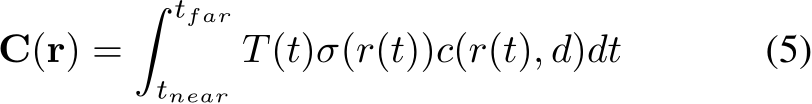
where C(r) is the final color of the ray r, T(t) = 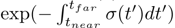is check the occlusion through the ray traveling from the near plane to the far plane and r(t) = o + td is the ray equation with origin o and direction d.

To train the MLP, NeRF uses a combination of coarse and fine rendering losses. The reconstruction loss measures the difference between the rendered color and the ground-truth color for each pixel in the training images. The total loss is defined as:

where r is the ray that passes through the pixel, is the ground truth color of the pixel. By minimizing this loss, the MLP learns to represent the scene as a neural radiance field that can synthesize novel views from any camera pose.

B. Neural Compression

There has also been an increased focus on using MLPs for Neural Compression, where MLPs aim to learn non-linear mapping as a function approximation to compress data and preserve the most relevant information. To this end, the MLP can be used as the encoder and/or the decoder in the compression pipeline. The encoder transforms the original data into a compressed representation, and the decoder aims to reconstruct the data. MLPs can be optimized to minimize the difference between the original and the reconstructed image. The loss function for neural data compression can be defined as:

where x is the original image, is the reconstructed image, z is the representation, D is a distortion measure such as mean squared error, R is a rate measure such as entropy, and is a trade-off parameter that balances the distortion and the rate.

C. Partial Differential Equations (PDEs)

Partial Differential Equations (PDEs) have attracted much attention recently. However, solving PDEs analytically is often impossible or impractical, and numerical methods can be costly or inaccurate.

MLPs can be used to solve PDEs in a data-driven and physics-informed way. One of the approaches is to use Physics-Informed Neural Networks (PINNs), which leverage MLPs to learn and approximate the solutions to complex physical systems. Given the underlying PDE and initial, boundary conditions embedded in a loss function, a coordinate-based neural network is trained to approximate the desired solution. PINNs take the form of:

where u(x, t) is the unknown solution, is an MLP with parameters is the spatial variable, and t is the temporal variable. The MLP is trained to satisfy the boundary and initial conditions of the PDE, as well as the PDE itself. The loss function can be defined as:

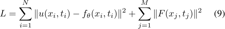
where N is the number of data points, M is the number of collocation points, is the observed or prescribed value of the solution at is the predicted value of the solution at , and is the residual of the PDE at , which is computed by applying automatic differentiation to the MLP. By minimizing this loss, the MLP learns to approximate the solution of the PDE that is consistent with the data and the physics.